Introduction

I put together these combinatorics notes while preparing for the Lanqiao Cup National Finals.

It started with ABC458 E. I realized that although I could derive the correct formula, I did not know how to evaluate it. I was unfamiliar with multiplicative inverses, Fermat’s little theorem, division in modular arithmetic, and several common combinatorial counting models. After working through that problem, I followed this thread with a systematic set of practice problems covering binomial-coefficient templates, a linear recurrence for inverses, derangements, the binomial theorem, the reflection principle, and Catalan numbers. (For my ABC458 E solution, see my other post: AtCoder ABC458-E Review: Separators, Nonempty Groups, and Vandermonde’s Convolution.)

This is not an encyclopedia of combinatorics. I will not develop Lucas’s theorem, the extended Euclidean algorithm, the Chinese remainder theorem, or more complicated inclusion–exclusion models. Its scope is clear: collect the combinatorics fundamentals that can turn into contest points.

I therefore focus on three questions:

1. How should division in modular arithmetic actually be handled?
2. How can common combinatorial counting models be translated quickly into formulas?
3. Which implementation details most often cause mistakes with boundaries, modular operations, or intermediate overflow?

Modular Division and Multiplicative Inverses

In ordinary mathematics, division is a natural operation. For example:

In modular arithmetic, however, we cannot simply write:

1

(a / b) % MOD

Integer division truncates, and “divide by $b$” modulo a number should mean “multiply by the multiplicative inverse of $b$,” rather than ordinary division.

Definition of a Multiplicative Inverse

If there is an integer $x$ satisfying:

Note: $\equiv$ means “is congruent to,” which can be understood as equality modulo $MOD$. In other words, $bx$ and $1$ have the same remainder when divided by $MOD$. Equivalently, $bx-1$ is divisible by $MOD$.

then $x$ is called the multiplicative inverse of $b$ modulo $MOD$, written:

Thus:

In code:

1

ans = a * inv(b) % MOD;

Remember that $0$ has no inverse, because no $x$ can satisfy:

The left-hand side is always $0$.

Finding Inverses with Fermat’s Little Theorem

If $MOD$ is prime and $a$ is not a multiple of $MOD$, Fermat’s little theorem gives:

Multiplying both sides by $a^{-1}$ gives:

Therefore, when $MOD$ is prime and $a \not\equiv 0 \pmod {MOD}$:

In code, we usually take its least nonnegative remainder in $[0,MOD-1]$:

The code is:

1
2
3
4
5
6
7
8
9
10
11
12
13
14
15
16
17
18
19
20
21

using ll = long long;

//快速幂模板
ll qpow(ll a, ll b) {
    ll res = 1;
    a %= MOD;
    while (b) {
        if (b & 1) {
            res = res * a % MOD;
        }
        a = a * a % MOD;
        b >>= 1;
    }
    return res;
}                           

//费马小定理求逆元
ll inv(ll a) {
    return qpow(a, MOD - 2);
}

The two comments in this template label binary exponentiation and inverse calculation using Fermat’s little theorem, respectively.

Common prime moduli include 1000000007 and 998244353.

Some problems also specify other particular prime moduli.

Conditions for Use

The conditions for using Fermat’s little theorem to find inverses are:

1. $MOD$ is prime;
2. The value $a$ whose inverse is needed is coprime to $MOD$;
3. Under a prime modulus, $a\not\equiv 0\pmod {MOD}$ guarantees that an inverse exists.

If the modulus is not prime, or $a$ is not coprime to it, we cannot blindly use:

1

qpow(a, MOD - 2)

That is a more general inverse problem, usually requiring tools such as the extended Euclidean algorithm. I will not cover it here.

A Linear Recurrence for Inverses of Individual Integers

If we need the inverse of every integer in $1\sim n$, we can of course write this for each $i$:

1

inv[i] = qpow(i, MOD - 2);

But the complexity is:

For large $n$, such as $3\times 10^6$, that is less efficient than we would like.

With a prime modulus, a linear recurrence can find all the inverses of individual integers in $O(n)$ time.

The recurrence starts with:

For $i\ge 2$:

Here, $inv_i$ denotes the multiplicative inverse of $i$ modulo $MOD$.

The point of this section is to understand where the formula comes from.

Why inv[0] Does Not Need Initialization

The meaning of an individual inverse inv[i] is:

When $i=0$, this becomes:

This is clearly impossible, so $0$ has no inverse.

The first meaningful entry in the array is therefore:

1

inv[1] = 1;

because:

Deriving the Recurrence

Suppose we want the inverse of $i$. Integer division gives:

For convenience, write:

Then:

Modulo $MOD$, we have $MOD\equiv 0$, so:

Rearranging:

That is:

Next, multiply both sides by the inverse of $r$, namely $inv[r]$.

Since:

we have:

Rearranging gives:

This shows that:

is the inverse of $i$.

Substitute back for $q$ and $r$:

To avoid a negative value, write:

This is the formula in the code:

1

inv[i] = (MOD - MOD / i) * inv[MOD % i] % MOD;

Why We Can Compute in Increasing Order

Since:

computing inv[i] uses inv[MOD % i], whose index is always smaller than $i$.

Starting from inv[1] and proceeding forward therefore ensures that every required value has already been computed.

Here is the handwritten derivation:

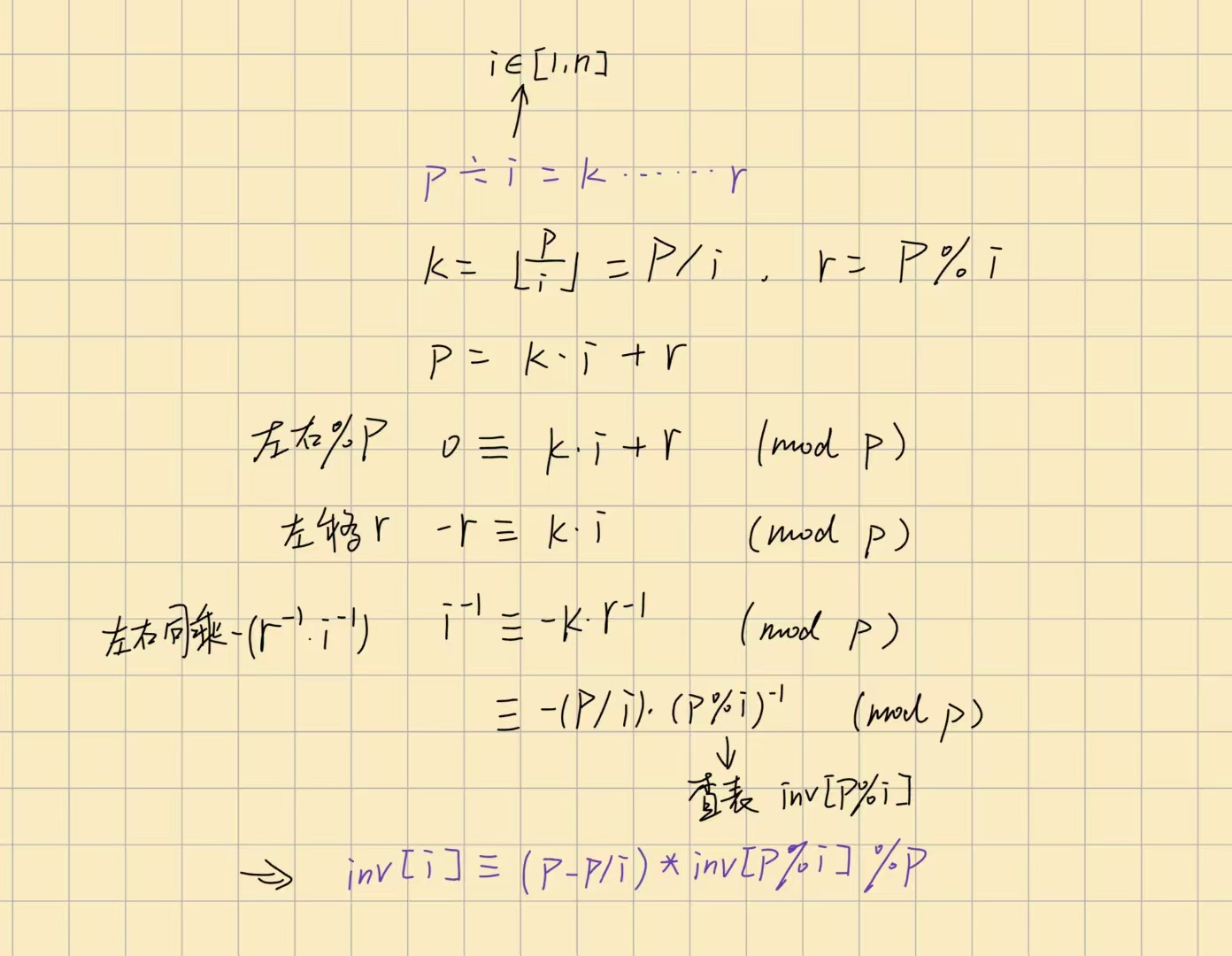
Image legend: $P$ denotes the modulus, $k$ the integer quotient, and $r$ the remainder. 左右%P means “reduce both sides modulo $P$”; 左移r means “move $r$ to the left”; 左右同乘 means “multiply both sides by the same expression”; 查表 means “look up the precomputed value.” The bottom line is the resulting recurrence for inv[i].

Template

1
2
3
4

inv[1] = 1;
for (int i = 2; i <= n; ++i) {
    inv[i] = (MOD - MOD / i) * inv[MOD % i] % MOD;
}

This linear recurrence computes inverses of individual integers:

Do not confuse them with inverse factorials.

Precomputing Factorials and a Binomial-Coefficient Template

The binomial-coefficient formula is:

In modular arithmetic, division becomes multiplication by inverses, so:

We can therefore precompute:

1
2

fac[i]  = i!
ifac[i] = (i!)^{-1}

and then evaluate binomial coefficients quickly.

The Factorial Array

The factorial array is straightforward:

1
2
3
4

fac[0] = 1;
for (int i = 1; i <= N; ++i) {
    fac[i] = fac[i - 1] * i % MOD;
}

Here:

The Inverse-Factorial Array

The inverse-factorial array represents:

First compute the largest entry:

1

ifac[N] = qpow(fac[N], MOD - 2);

Notice that this uses:

1

qpow(fac[N], MOD - 2)

rather than:

1

qpow(N, MOD - 2)

because ifac[N] represents $(N!)^{-1}$, not $N^{-1}$.

Then work backward.

Since:

we have:

That is:

In code:

1
2
3

for (int i = N - 1; i >= 0; --i) {
    ifac[i] = ifac[i + 1] * (i + 1) % MOD;
}

Binomial-Coefficient Template

1
2
3
4
5
6

ll C(int n, int k) {
    if (k < 0 || k > n) {
        return 0;
    }
    return fac[n] * ifac[k] % MOD * ifac[n - k] % MOD;
}

The complete preprocessing template is:

1
2
3
4
5
6
7
8
9
10
11
12
13
14
15
16
17
18
19
20
21
22
23
24
25
26

long long qpow(long long a, long long b) {
    long long res = 1;
    a %= MOD;
    while (b) {
        if (b & 1) res = res * a % MOD;
        a = a * a % MOD;
        b >>= 1;
    }
    return res;
}

void init(int N) {
    fac[0] = 1;
    for (int i = 1; i <= N; ++i) {
        fac[i] = fac[i - 1] * i % MOD;
    }
    ifac[N] = qpow(fac[N], MOD - 2);
    for (int i = N - 1; i >= 0; --i) {
        ifac[i] = ifac[i + 1] * (i + 1) % MOD;
    }
}

long long C(int n, int k) {
    if (k < 0 || k > n) return 0;
    return fac[n] * ifac[k] % MOD * ifac[n - k] % MOD;
}

Limits of Applicability

This template applies when:

1. $MOD$ is prime;
2. The largest precomputed $N$ is not too large;
3. The ordinary factorials do not encounter the more complicated case $n\ge MOD$.

If $n$ is enormous, or factorials contain a factor of the modulus once $n\ge MOD$, this template cannot simply be applied as is. Those are more general topics involving tools such as Lucas’s theorem, which I will not cover here.

The Derangement Model

A derangement asks: given $n$ elements, how many permutations place no element back in its original position?

Denote the number of derangements by:

The usual initial values are:

The recurrence is:

Deriving the Recurrence

Consider the $n$th element.

It cannot occupy its own position, so it can occupy any of the first $n-1$ positions. Suppose we place it at position $k$, where:

Next, consider the element originally belonging to position $k$.

Call the $k$th element $k$.

After placing $n$ at position $k$, there are two cases for element $k$.

Case 1: Element k Goes to Position n

In other words, $k$ and $n$ exchange positions.

The positions of these two elements are now fixed:

• $n$ occupies $k$'s position;
• $k$ occupies $n$'s position.

The remaining $n-2$ elements must still all be deranged, giving:

Case 2: Element k Does Not Go to Position n

We can now regard position $n$ as the forbidden position corresponding to $k$.

In other words, after removing element $n$, the remaining $n-1$ elements still form a derangement problem: each element must avoid its corresponding forbidden position.

This contributes:

The $n$th element has $n-1$ possible positions, so the total is:

Template

1
2
3
4
5

D[0] = 1;
D[1] = 0;
for (int i = 2; i <= N; ++i) {
    D[i] = (i - 1) * (D[i - 1] + D[i - 2]) % MOD;
}

If the problem does not require a modulus and the bounds are small, % MOD can be omitted.

Combining Derangements with Binomial Coefficients

A common variant asks for permutations with exactly $m$ fixed positions.

First choose those $m$ fixed positions:

None of the remaining $n-m$ positions may be fixed, so they form a derangement problem:

The answer is therefore:

Luogu P4071 is a typical application of this model.

The Binomial Theorem and Coefficient Problems

The basic form of the binomial theorem is:

One way to understand it is:

There are $k$ factors, and we choose either $A$ or $B$ from each. Choosing $A$ exactly $i$ times means choosing $B$ exactly $k-i$ times. There are $C_{k}^{i}$ such choices.

Binomials with Coefficients

Suppose the expression is:

and we want the coefficient of the term:

To obtain $x^n$, we must choose $ax$ exactly $n$ times; to obtain $y^m$, we must choose $by$ exactly $m$ times. The problem usually guarantees:

Choosing which $n$ of the $k$ factors supply $ax$ gives:

Each choice of $ax$ contributes one factor of $a$, so $n$ such choices contribute:

Each choice of $by$ contributes one factor of $b$, so $m$ such choices contribute:

The final coefficient is therefore:

Equivalently:

since $n+m=k$.

In Code

1

ans = C(k, n) * qpow(a, n) % MOD * qpow(b, m) % MOD;

Two easy mistakes are calculating only the binomial coefficient and using $C_{n}^{m}$ as the binomial coefficient.

The key to Luogu P1313 is translating the polynomial-coefficient question in the statement into this formula.

The Reflection Principle and Generalized Catalan Counting

The reflection principle is a classic way to handle constraints requiring every prefix to remain valid.

A common model is:

Given $n$ copies of 1 and $m$ copies of 0, count the strings in which every prefix contains at least as many 1s as 0s.

That is, every prefix must satisfy:

Total Number of Strings

Ignoring the prefix constraint, choose $m$ of the $n+m$ positions for 0, and fill the rest with 1.

The total number of strings is therefore:

Characterizing Invalid Strings

An invalid string has some prefix satisfying:

Scan an invalid string from left to right and consider the first position where it becomes invalid.

At that position, we must have:

Only one character is added at a time, so the difference cannot jump over this state.

Reflecting the First Prefix That Crosses the Boundary

For an invalid string, find the first prefix satisfying:

Swap every 0 and 1 in that prefix.

Suppose the prefix originally contains $a$ copies of 1 and $a+1$ copies of 0:

After reflection, it contains $a+1$ copies of 1 and $a$ copies of 0:

The totals in the whole string therefore change from $n$ copies of 1 and $m$ copies of 0:

to $n+1$ copies of 1 and $m-1$ copies of 0:

Thus, every invalid string maps to an unrestricted string containing $n+1$ copies of 1 and $m-1$ copies of 0.

Why This Is a Bijection

Proving a mapping in one direction is not enough; we must also show that it neither overcounts nor misses anything.

Conversely, take any string containing $n+1$ copies of 1 and $m-1$ copies of 0:

Scan it from left to right and find the first prefix satisfying:

This prefix must exist: the whole string has one more 1 and one fewer 0 than before. In terms of the prefix difference, the final difference must become positive, so it must reach $+1$ for the first time somewhere.

Then swap every 0 and 1 in this prefix.

The prefix originally contains $a+1$ copies of 1 and $a$ copies of 0:

After reflection, it contains $a$ copies of 1 and $a+1$ copies of 0:

The reflected string therefore first reaches:

at this prefix, making it an invalid string.

The operations in the two directions are inverses:

• Reflect an invalid string at the first point where its difference falls to $-1$, obtaining a string of the other, unrestricted kind;
• Reflect that unrestricted string at the first point where its difference rises to $+1$, returning to the invalid string.

The number of invalid strings is therefore:

The Generalized Formula

The number of valid strings is thus:

If $n<m$, even the entire string has fewer 1s than 0s, so every prefix cannot possibly have at least as many 1s as 0s. The answer is directly $0$.

Luogu P1641 is a typical problem using this model.

Standard Catalan Numbers and Pitfalls Without a Modulus

Setting $n=m$ in the previous section gives the standard Catalan-number model.

That is:

Given $n$ copies of 1 and $n$ copies of 0, require every prefix to contain at least as many 1s as 0s.

The reflection-principle formula gives:

This is one form of the $n$th Catalan number.

It also simplifies to:

Here is a short derivation. Since:

and:

the ratio is:

In other words:

Substitute back into the original expression:

to obtain:

From the Binomial-Coefficient Formula to a Recurrence

If there is no modulus and $n$ is small, we can compute Catalan numbers directly with a linear recurrence, avoiding intermediate factorial overflow.

Starting from:

and:

consider their ratio:

Rearranging gives:

where:

Thus:

After simplification:

The recurrence is therefore:

In code:

1
2
3
4

cat[0] = 1;
for (int i = 1; i <= n; ++i) {
    cat[i] = cat[i - 1] * (4 * i - 2) / (i + 1);
}

Here is the handwritten derivation:

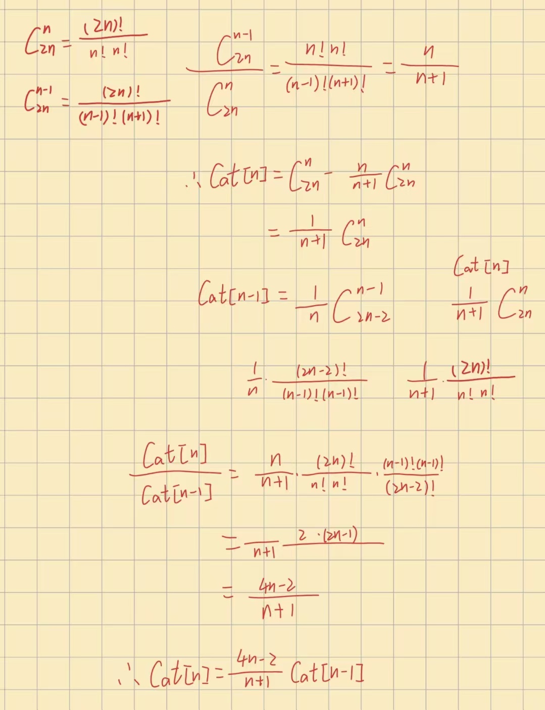
Image guide: the top section compares the two binomial coefficients, the middle obtains the standard Catalan formula, and the bottom takes the ratio of consecutive Catalan numbers to derive the recurrence. The notation matches the formulas above.

The Pitfall When Computing Without a Modulus

In Luogu P1754, $n\le 20$, and the final answer fits in long long.

But directly using factorials to calculate:

requires computing up to:

When $n=20$, an intermediate value is:

This is far beyond the range of long long.

The pitfall here is therefore about intermediate values rather than the final answer:

A final answer that fits does not guarantee that intermediate factorials fit.

In this situation, use the Catalan recurrence, a more reliable multiplicative formula for binomial coefficients, or arbitrary-precision arithmetic.

Common Pitfalls

This section collects the places in this topic where it is easiest to make a coding or reasoning mistake.

Distinguish Individual Inverses, Inverse Factorials, and Factorials

The three arrays most easily confused are:

1
2
3

fac[i]  = i!
ifac[i] = (i!)^{-1}
inv[i]  = i^{-1}

Their meanings are entirely different.

fac[i] is a factorial:

ifac[i] is the inverse of a factorial:

inv[i] is the inverse of the individual integer $i$:

The binomial-coefficient template uses:

1

fac[n] * ifac[k] % MOD * ifac[n - k] % MOD

Ordinary modular division uses:

1

a * inv[b] % MOD

Do Not Confuse Forward inv with Backward ifac

The linear recurrence for individual inverses proceeds forward:

1
2
3
4

inv[1] = 1;
for (int i = 2; i <= n; ++i) {
    inv[i] = (MOD - MOD / i) * inv[MOD % i] % MOD;
}

It computes:

The inverse-factorial recurrence proceeds backward:

1
2
3
4

ifac[N] = qpow(fac[N], MOD - 2);
for (int i = N - 1; i >= 0; --i) {
    ifac[i] = ifac[i + 1] * (i + 1) % MOD;
}

It computes:

Both formulas involve inverses, but they calculate fundamentally different things.

Add MOD for Modular Subtraction

If the answer contains a subtraction, such as:

write it modulo the modulus as:

1

(a - b + MOD) % MOD

Otherwise, even when the actual answer is nonnegative, the first reduced value may be smaller than the second, causing a negative output.

In Luogu P1641, the formula is:

Subtracting directly can produce WA.

0 Has No Inverse

No $x$ satisfies:

so inv[0] has no meaning.

When finding individual inverses with a linear recurrence, start at inv[1].

Inverses via Fermat Require a Prime Modulus

1

qpow(a, MOD - 2)

This expression relies on Fermat’s little theorem, so $MOD$ must be prime and $a$ must not be a multiple of $MOD$.

For a nonprime modulus, we need more general methods for determining whether an inverse exists and computing it. Those are beyond this article.

A Final Answer That Fits Does Not Guarantee Intermediate Factorials Fit

In combinatorial counting without a modulus, checking only the final answer’s range is insufficient.

For example, in Luogu P1754, the final answer fits in long long, but calculating binomial coefficients with factorials produces $40!$ as an intermediate value and immediately overflows.

Use a different calculation method in such cases, such as the Catalan recurrence.

Use the Correct Variables in Binomial Coefficients

It is especially easy to mix up variables in binomial-coefficient problems.

For example, Luogu P1313 asks for the coefficient of $x^n y^m$ in:

The correct binomial coefficient is:

rather than:

because we are choosing $n$ of the $k$ factors from which to take $ax$.

Precompute Through the Largest Index the Problem Needs

If the problem requires:

the preprocessing range must reach at least:

Do not stop at only $n$ or $m$.

For example, grid-path problems such as Luogu P2265 need:

Prefix-Validity Problems Have No Solution When n < m

Consider the model:

Given $n$ copies of 1 and $m$ copies of 0, require every prefix to contain at least as many 1s as 0s.

If:

the whole string already contains fewer 1s than 0s. The condition is impossible, so the answer is directly $0$.

Practice Log

These are the practice problems used in this topic. I do not expand their solutions here; I only note what each one trains and link to the accepted code.

• Luogu B2164: Basic binomial coefficients and modular arithmetic. Accepted code

• Luogu B3717: Practice involving multiplicative inverses and binomial coefficients. Accepted code

• Luogu P2265: Grid-path counting; modeling with $C_{n+m}^{n}$ and using the binomial-coefficient template. Accepted code

• Luogu P4071: Fixed-point counting and derangements; practicing $C_{n}^{m}\cdot D(n-m)$. Accepted code

• Luogu P1595: The basic derangement model and the recurrence for $D_n$. Accepted code

• Luogu P3811: A linear recurrence for inverses of individual integers. Accepted code

• Luogu P1313: The binomial theorem and evaluating coefficients of terms with scalar factors. Accepted code

• Luogu P1641: The reflection principle and generalized Catalan counting. Accepted code

• Luogu P1754: Standard Catalan numbers and intermediate-factorial overflow when no modulus is used. Accepted code

• ABC458 E: Combining a combinatorial formula derivation, separator modeling, and modular inverses. Accepted code

Closing Thoughts

These notes collect the combinatorics fundamentals I filled in while preparing for the Lanqiao Cup.

Starting with modular division, multiplicative inverses answer how to divide modulo a number. Fermat’s little theorem and binary exponentiation provide the basic tools for finding inverses under a prime modulus. A linear recurrence extends this to finding individual inverses in bulk, while precomputed factorials and inverse factorials form the basis of the binomial-coefficient template.

At the modeling level, derangements, the binomial theorem, the reflection principle, and Catalan numbers each cover common kinds of combinatorial counting problems. What matters is remembering how a statement turns into these models, rather than remembering the code for one particular problem:

• Fixed points and elements avoiding their original positions suggest derangements;
• The coefficient of a specified term in a polynomial expansion suggests the binomial theorem;
• Prefix-validity constraints in paths, parentheses, queues, and binary strings suggest the reflection principle;
• Prefix-validity problems with equal counts lead to standard Catalan numbers.

This is far from all of combinatorics, but for contests such as the Lanqiao Cup, it already covers many basic models that can translate directly into points. If I encounter more general counting problems later, I can add Lucas’s theorem, the extended Euclidean algorithm, or more complicated inclusion–exclusion as needed. At this stage, getting these basic templates and derivations solid matters more than expanding the list blindly.