Introduction
I’ve recently been taking a course on Agentic AI. One lecture, Post-Training Verifiable Agents, gave me a basic understanding of concepts such as agent, tool, harness, verifier, and reward, along with an introductory grasp of methods including SFT, RL, Best-of-N, and Rejection Sampling. But I hadn’t actually run the whole system myself.
So I decided to do a Lab to reinforce what I’d learned. There were two main things I wanted to understand: how much difference there would be between One-shot inference and an Agent Loop using the same LLM, and how much Test-time Sampling would improve the Agent Loop as I added more rollouts. I used SWE-bench Lite as the benchmark.
1. Pilot: preparing the experiment
1.1 Experimental framework and design
The experiment called the Deepseek-V4-Flash Thinking model.
A was the One-shot baseline. The model received an issue and roughly 13K tokens of static repository context retrieved with BM25. It made a single API request, used no tools, received no environmental feedback, and directly output a Patch. This measured the same model’s ability to produce a repair in one go using only fixed context.
B was an Agent Loop with access to list_tree, read_file, search_code, edit_file, write_file, run_shell, and finish. The harness returned each execution result to the model as an Observation. The model could then continue reasoning, editing, or testing until it called finish itself or reached the step limit.
Each SWE-bench Lite task provided a real issue and the corresponding repository’s Base Commit. A and B both ultimately produced a Candidate Patch, which the official verifier evaluated in an isolated evaluation environment to determine whether the task was solved. B’s Agent Loop itself ran in a separate Docker container.
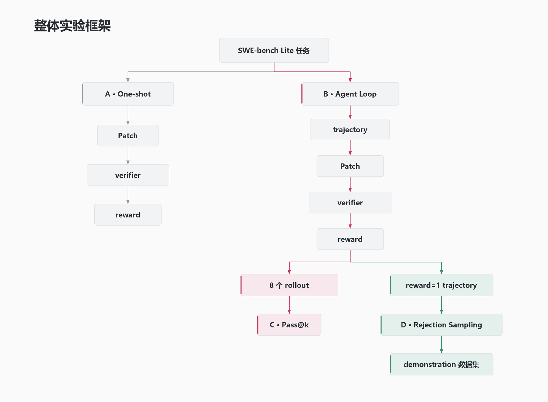
A and B share the task set; Pass@k comes from repeated B rollouts, and Rejection Sampling processes only successful trajectories.
Diagram guide: SWE-bench Lite tasks branch into A · One-shot → Patch → verifier → reward, and B · Agent Loop → trajectory → Patch → verifier → reward. Eight B rollouts feed C · Pass@k; reward=1 trajectories feed D · Rejection Sampling and then a demonstration dataset.
A and B were parallel method comparisons. C evaluated repeated B rollouts, while D processed trajectories that had already finished. The four parts shared tasks and artifacts; a single trajectory did not pass sequentially from A through D.
C ran 8 independent B rollouts for each task and calculated Pass@1, Pass@2, Pass@4, and Pass@8. Rollouts shared neither conversations nor workspaces. This measured how many tasks the candidate set could cover as sampling increased.
D was offline Rejection Sampling. It retained B trajectories with reward=1, rejected those with reward=0, and then deduplicated Patches within each task to produce data that could be used later.
1.2 Agent Loop and Test-time Sampling
The Agent Loop ran in a separate container without network access or mounted host directories. Every rollout started from the same Base Commit. Its workspace did not inherit the previous Patch, and it could not see other rollouts’ trajectories. The official evaluator ran only after the agent finished. This kept the Gold Patch, earlier sampling results, and evaluation details separate. The Gold Patch was used to confirm that the benchmark and evaluation environment worked; it can be understood as the official answer, and was never included in the prompt, workspace, or information returned by tools.
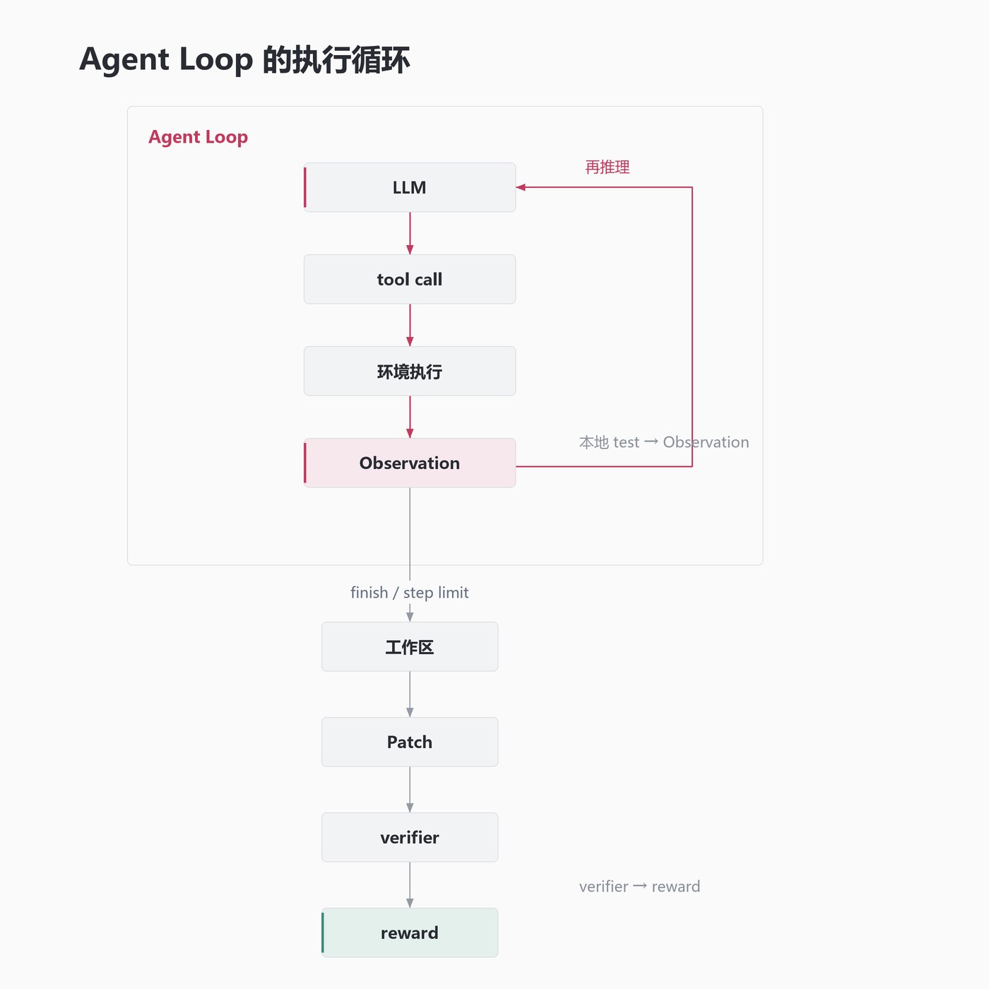
local test results return as Observations; the final verifier supplies the reward after the loop ends.
Diagram guide: LLM → tool call → execution in the environment → Observation → further reasoning. At finish or the step limit, the workspace yields a Patch for the verifier, which returns a reward. Local tests feed Observations, not the final reward.
Passing local tests through run_shell did not mean a task had earned reward=1. Local tests might provide incomplete coverage, and later edits could break behavior that had previously passed. The experiment recognized only the verifier result for the final Candidate Patch.
1.3 Pilot v1
Pilot v1 started with four tasks and returned A=0/4 and B=1/4. After checking the trajectories and logs, I found that these two numbers weren’t directly comparable.
At the time, A had max_tokens set to 8192, with reasoning and the final answer sharing that output budget. Of the four One-shot runs, 3/4 hit the token limit, and 4/4 final Patches were empty. The token limit was too low.
B’s problem was more straightforward: all 15 calls to apply_patch failed, and 4/4 B trajectories hit the 30-step limit. Even when the model found the right location, it had no reliable editing interface.
With all of A’s Patches empty and B’s editing interface broken, there was no point continuing to compare 0/4 with 1/4. I moved straight on to Pilot v2.
1.4 Pilot v2: fixing the harness and validating the protocol
Pilot v2 first addressed the problems exposed by Pilot v1. I raised One-shot’s max_tokens from 8192 to 65536. B stopped using apply_patch and switched to edit_file and write_file; its step limit also rose from 30 to 60. The goal of this round was to confirm that A and B could run properly, not to chase a higher score.
After repairing the interfaces, I checked B’s diversity. I ran 4 independent B rollouts on the same Astroid task. They took 39, 26, 40, and 34 steps and produced 4 different Patch hashes. They used the same Base Commit, prompt, model, and harness configuration, with isolated containers. This was only a diversity check, not a Pass@k calculation. It confirmed that the same model could produce different trajectories on the same task.
All four One-shot runs in Pilot v2 produced nonempty Patches, with no further output truncation. All four main B trajectories called finish themselves, none reached the 60-step limit, and edit_file produced no errors. At this point, the harness was basically stable and ready for the Formal phase.
1.5 Freezing the experimental protocol
Formal used 20 tasks from 10 repositories, with two tasks per repository. A ran once per task and B ran 8 times, producing 20 A trajectories and 160 B trajectories: 180 formal trajectories in total.
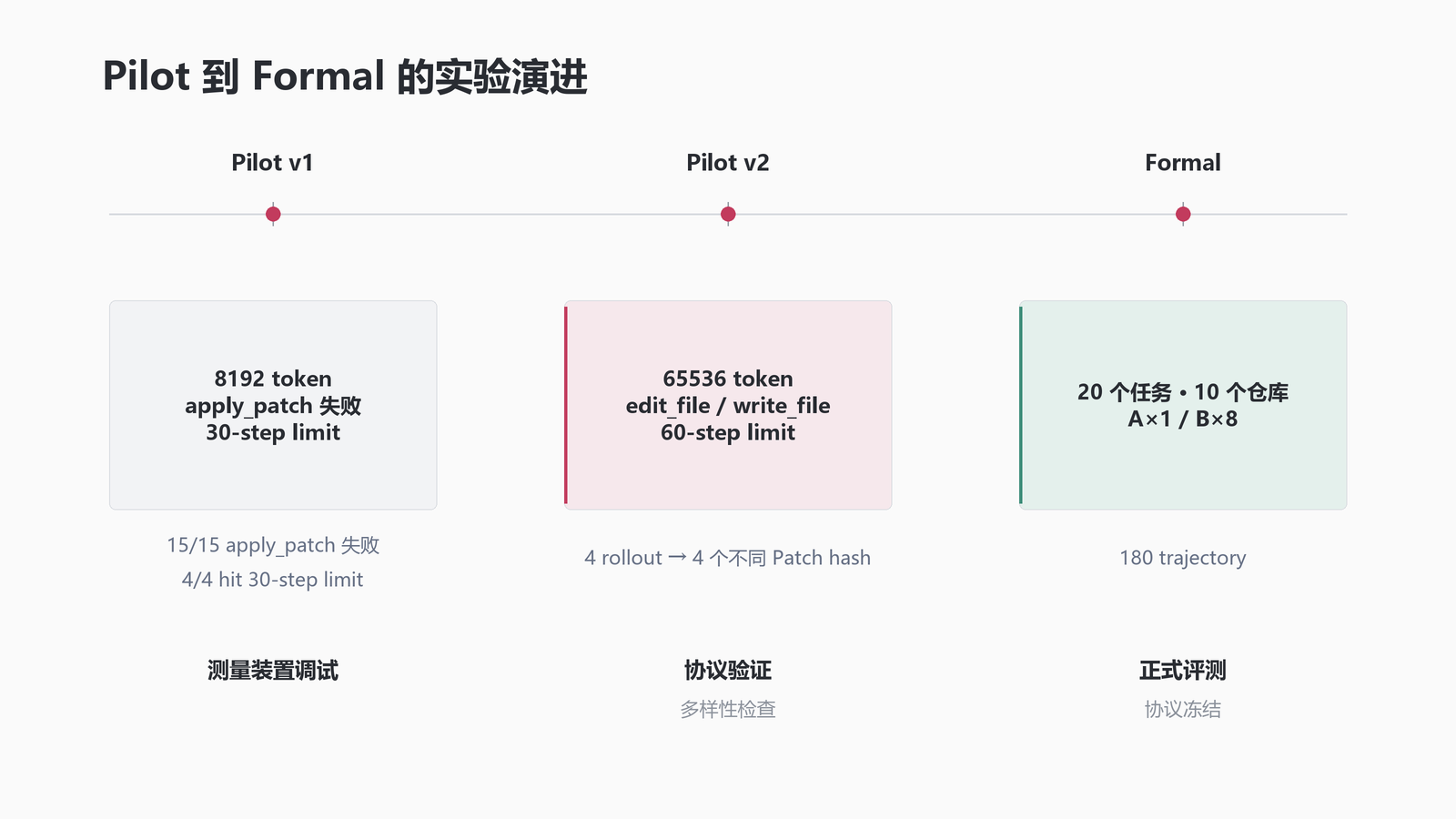
Pilot v1 exposed harness problems; Pilot v2 validated the corrected protocol; Formal ran with frozen settings. Scores from the three stages are not pooled.
Diagram guide: Pilot v1—8192 tokens, failed apply_patch, 30-step limit, measurement setup debugging. Pilot v2—65536 tokens, edit_file / write_file, 60-step limit, protocol validation and diversity checks. Formal—20 tasks, 10 repositories, A×1 / B×8, 180 trajectories, frozen protocol.
| Item | One-shot | Agent Loop |
|---|---|---|
| Runs per task | 1 | 8 independent rollouts |
| Repository information | Roughly 13K tokens of static BM25 repository context | Active workspace retrieval through tools |
| Environment interaction | None | Read and write code, run commands, receive Observations |
| Editing method | Directly output the final Patch | edit_file / write_file |
| Termination | End of one API request | finish or the 60-step limit |
| Final judgment | Verifier | The same verifier |
Before entering Formal, I froze the model, prompt, tools, max_steps, token budgets, verifier, reward classification rules, and task set. Changing the prompt, adding steps, or supplying more tools whenever a task failed would turn formal evaluation into continuous tuning against the benchmark. So even when a task scored 0/8, or a trajectory remained unfinished at step 60, I retained the original result and left changes for the next experiment.
One detail worth mentioning: at 20/180, Formal was interrupted by a failure to write a checkpoint on Windows. I made a fix limited to saving checkpoint state. I did not change the model, prompt, tools, steps, verifier, or reward, and did not rerun completed trajectories. After the fix, the same Formal run continued with protocol_changed=false.
2. Results
2.1 One-shot versus Agent Loop: 20% vs 55%
The Formal results were clear: One-shot solved 4/20 tasks, or 20%. Of the Agent Loop’s 160 rollouts, 88 succeeded, giving a task-averaged Pass@1 of 55%. The difference was 35 percentage points.
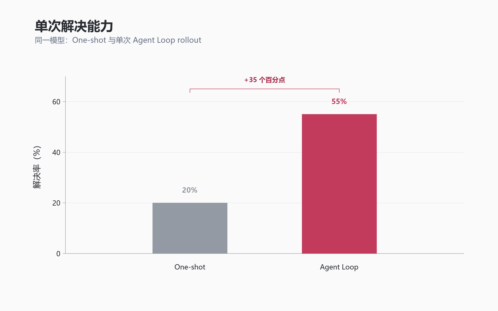
on the same 20 tasks, One-shot achieved 20% and Agent Loop Pass@1 reached 55%.
Chart guide: the vertical axis is resolution rate (%); gray is One-shot and red is Agent Loop. The bracket marks a 35-percentage-point difference for the same model.
One-shot saw only static repository context. The Agent Loop could inspect code, edit, test, and adjust its next actions using Observations. The 35-percentage-point difference came from this overall change in interaction, and cannot be attributed to an individual tool or a particular piece of test feedback. The comparison is also limited to this frozen set of 20 tasks.
Each task had 8 B rollouts, for 160 across 20 tasks, of which 88 had reward=1. Averaging c/8 across tasks also gives 88/160=55%. This happens to equal the success proportion across all trajectories, but Pass@1 is still defined by task. The subsequent Pass@2, Pass@4, and Pass@8 use the same calculation.
2.2 Pass@k
Formal sampled a fixed 8 rollouts per task. Let n=8, c be the number of successful rollouts, and k be the number of candidates drawn from the observed samples. When k=n=8, a task’s Pass@8 is 1 whenever c>0.
With more independent B rollouts, Pass@1, Pass@2, Pass@4, and Pass@8 were 55.00%, 61.7857%, 64.6429%, and 65.00%, respectively. Increasing from 1 candidate to 2 improved coverage by 6.79 percentage points; going from 2 to 4 added 2.86 points; going from 4 to 8 added only 0.36 points.
Specifically, when k=n=8, a task’s Pass@8 is 1 as long as c>0. In this experiment, 13/20 tasks succeeded at least once, so both average Pass@8 and Solved@8 were 65%.
| Metric | Result | What the number represents |
|---|---|---|
| One-shot | 20.00% (4/20) | Proportion of tasks solved with one static inference per task |
| Agent Loop Pass@1 | 55.00% | Estimated coverage by one candidate, derived from 8 measured rollouts per task |
| Agent Loop Pass@2 | 61.7857% | Estimated coverage where at least one of two candidates succeeds |
| Agent Loop Pass@4 | 64.6429% | Estimated coverage where at least one of four candidates succeeds |
| Agent Loop Pass@8 | 65.00% | Task coverage of the full 8-rollout candidate set observed here |
| Solved@8 | 65.00% (13/20) | Proportion of tasks with at least one success in 8 measured rollouts |
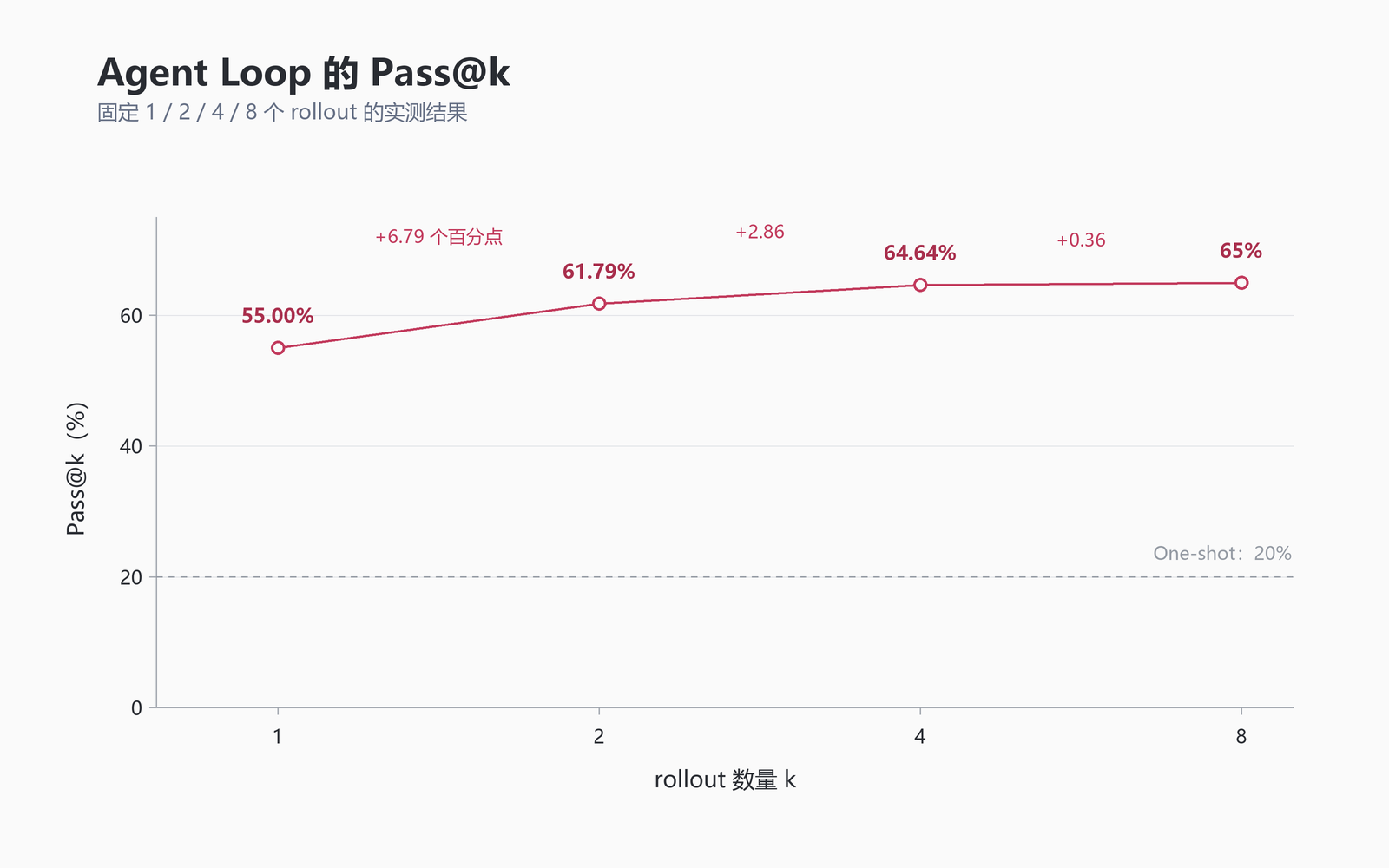
Test-time Sampling improved task coverage, but the gain from P@4 to P@8 was only 0.36 percentage points.
Chart guide: the horizontal axis is candidate/rollout count k; the vertical axis is Pass@k (%). Red annotations show gains in percentage points. The dashed gray line is One-shot at 20%.
Pass@k, Best-of-N, and Rejection Sampling serve different purposes. Pass@k asks whether a successful result exists among the candidates. Best-of-N additionally needs a selector to choose one of N candidates. Rejection Sampling uses a verifier to filter trajectories for data generation. This experiment had no selector, so Pass@8 cannot be treated directly as a deployment success rate.
2.3 Task-level c/8 and the gains from sampling
Breaking the aggregate curve down by task, 7 of the 20 tasks scored 0/8, another 7 scored 8/8, and only 6 fell between those extremes. Those 6 succeeded 3, 5, 5, 6, 6, and 7 times, respectively. No task scored 1/8 or 2/8.
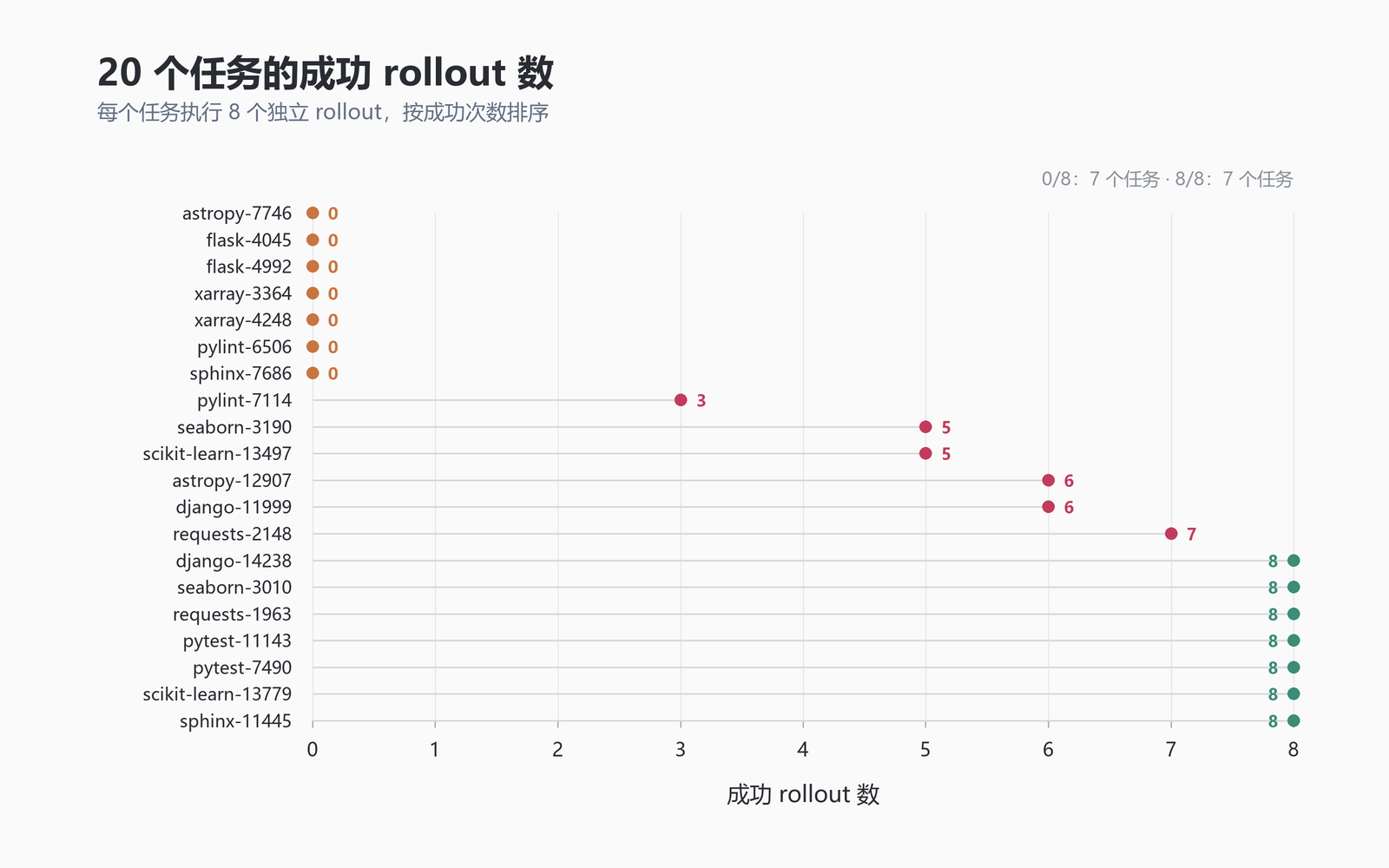
measured c/8 for each task; 7 tasks at each extreme and 6 in the middle.
Chart guide: each row is a task, ordered by successful rollout count on the horizontal axis. Orange marks 0/8, green marks 8/8, and red marks intermediate results. Each task has 8 independent rollouts.
This also explains why Pass@k saturated quickly. More samples could not increase coverage for the 7 tasks already at 8/8. The 7 tasks at 0/8 had no successes within the current 8 samples, so the additional gains mainly came from the 6 tasks in between. Here, 0/8 describes only what was observed in this experiment; it does not mean that further rollouts would necessarily be useless.
2.4 Steps and costs for successful and failed trajectories
Of the 160 B trajectories, 88 succeeded and 72 failed. Successful trajectories used a mean of 35.26 steps, with a median of 32. Failed trajectories used a mean of 45.5 steps, with a median of 52.5.
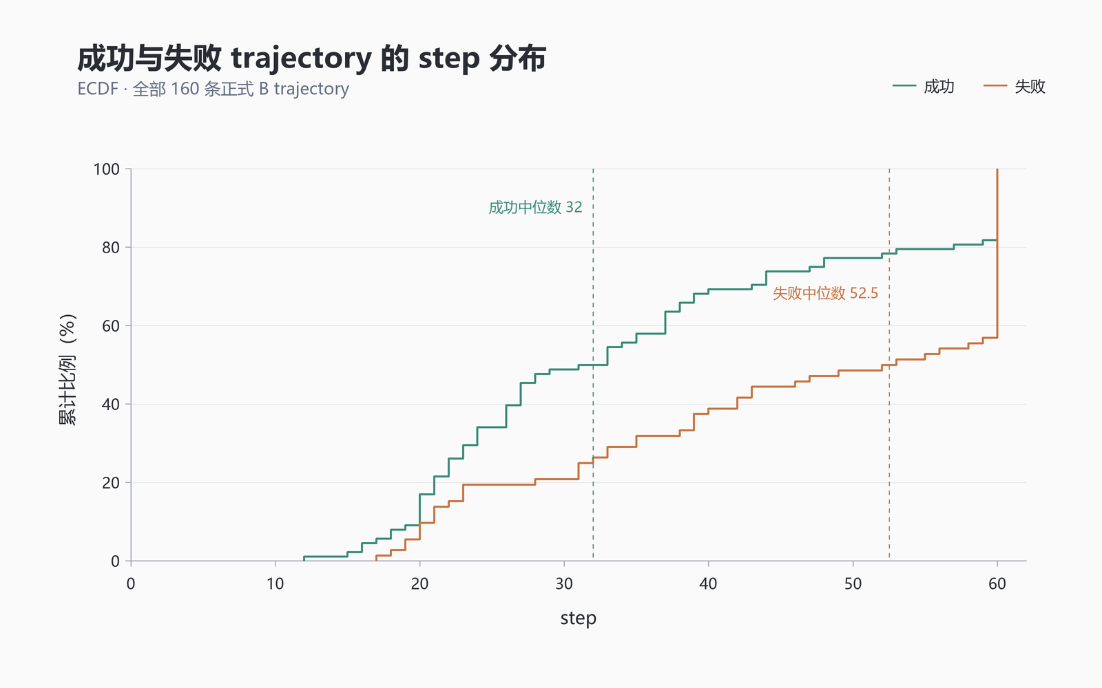
the median was 52.5 steps for failed trajectories and 32 for successful ones, a difference of 20.5 steps.
Chart guide: green means success and orange means failure. The horizontal axis is step count; the vertical axis is cumulative proportion (%). Dashed lines mark the two medians.
The ECDF (empirical cumulative distribution function) above includes every trajectory, with no smoothing or removal of extreme points. At any step position, it shows the proportion of trajectories that had ended by that point. The failure curve shifts right across the distribution as a whole; the difference is not just a few 60-step samples pulling up the mean.
Successful trajectories had a mean API cost of 0.06984 CNY and a median of 0.05082 CNY. Failed trajectories had a mean cost of 0.13955 CNY and a median of 0.11717 CNY. The failed group’s mean cost was about twice the successful group’s, and its median was more than twice as high. Costs across all samples ranged from 0.01028 to 0.39885 CNY, and the ECDF retains the high-cost tail.
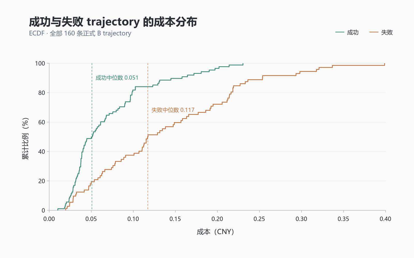
both mean and median cost were higher for failed trajectories than for successful ones.
Chart guide: green means success and orange means failure. The horizontal axis is cost (CNY); the vertical axis is cumulative proportion (%). The dashed median labels are rounded to 0.051 and 0.117 CNY.
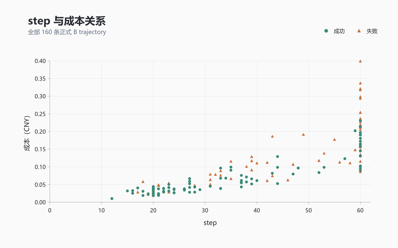
costs were usually higher at larger step counts, with substantial price variation even at the same number of steps.
Chart guide: the horizontal axis is step count and the vertical axis is cost (CNY). Green circles are successful trajectories; orange triangles are failed trajectories. All 160 formal B trajectories are included.
The scatter plot fills in the relationship between steps and cost. There are more failed points in the high-step region, but costs at the same step count still vary with input tokens, output tokens, and cache hits. This is a correlation; it does not establish that longer execution causes failure. Steps describe interaction length, while CNY records actual API consumption.
2.5 Differences in tool use
In average calls per trajectory, the failed group used read_file 15.03 times versus 9.64 for the successful group; search_code was 10.15 versus 6.09, edit_file was 4.43 versus 2.93, and run_shell was 22.92 versus 19.40. Failed trajectories also used list_tree more, while successful ones used write_file and finish slightly more.
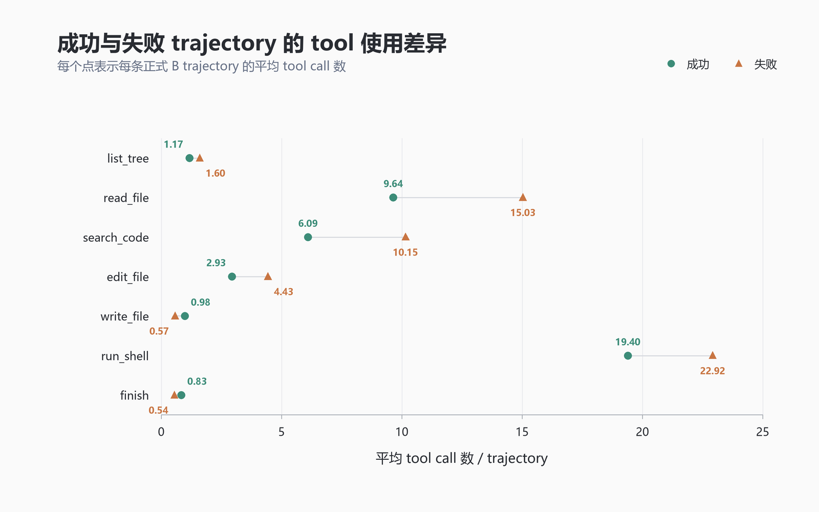
failed trajectories had higher average call counts for most tools.
Chart guide: the horizontal axis is average tool calls per trajectory. Green circles mean success and orange triangles mean failure; each row names a tool.
Failed trajectories tended to spend more calls searching, editing, and testing. Some of that was necessary investigation, and some was repeated reading and repeated Patch revisions. The fact that write_file and finish did not rise alongside the other counts also reminded me not to look only at totals. finish means the agent chose to stop; a read_file call might retrieve a crucial fact or merely reread the same code. Call order, arguments, and the Observations returned afterward tell us more than counts alone.
2.6 Step limits and outcomes
In Formal B, 46 trajectories reached the 60-step limit: 15 succeeded and 31 failed, a success rate of 32.61%. Of the 114 that did not reach it, 73 succeeded and 41 failed, a success rate of 64.04%.
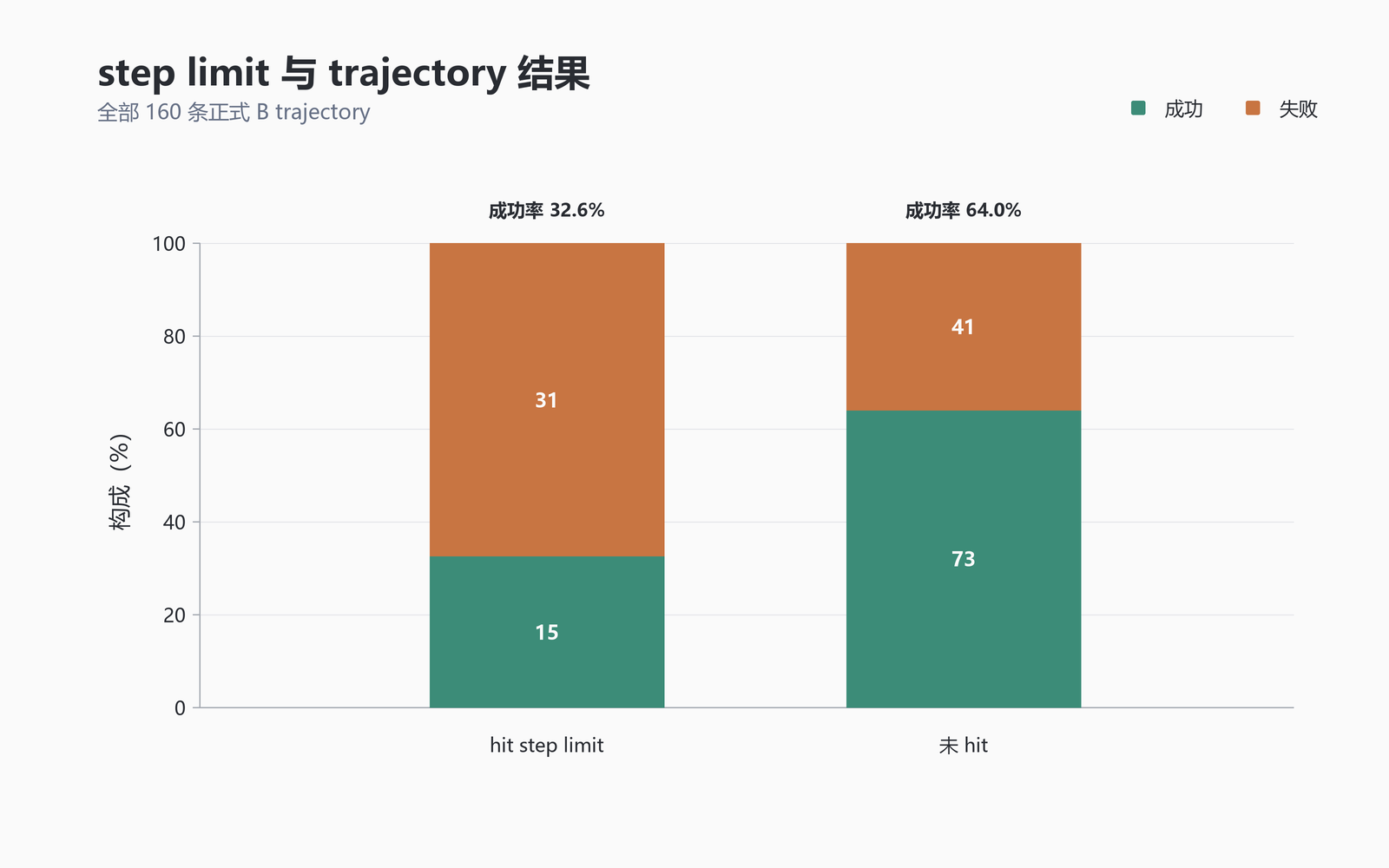
trajectories that reached the step limit had a success rate of 32.6%, versus 64.0% for those that did not.
Chart guide: the left bar reached the step limit; the right did not. Green is success and orange is failure. The vertical axis shows percentage composition; numbers inside the bars are trajectory counts.
There were still 15 successes among the 46 that reached the limit, and 41 failures among the 114 that did not. The step limit was associated with outcome, but it could not replace an examination of what happened within a trajectory.
Failed trajectories ran longer and cost more, and 46 trajectories hit the limit. This made me wonder whether 60 steps was too restrictive. The aggregates couldn’t tell me whether those trajectories were still making progress at the boundary or had already fallen into repeated searches, so I went on to inspect the 7 tasks with c=0.
3. Failure analysis of c=0 tasks
3.1 Classifying 56 failed trajectories
The 7 c=0 tasks each had 8 rollouts without a single success, giving 56 trajectories with reward=0. After Formal finished, I analyzed them individually. I mainly looked at whether the final Patch touched relevant code, whether there were new edits or new test feedback late in the run, and whether the trajectory showed repeated searching, back-and-forth Patch changes, or scope drift. This subset consists of tasks that remained unsolved across all 8 samples; it does not represent all 72 failed trajectories.
The classification was a retrospective, heuristic, qualitative judgment, not a ground-truth label supplied by the verifier. The analysis also did not randomly vary max_steps or replanning strategies. I classified the 56 trajectories as follows: 35 capability/semantic failures (likely_capability_failure), or 62.5%; 11 strategy failures (likely_strategy_failure), or 19.6%; 7 horizon-limited failures (likely_horizon_limited), or 12.5%; and 3 mixed/unclear cases (mixed_or_unclear), or 5.4%.
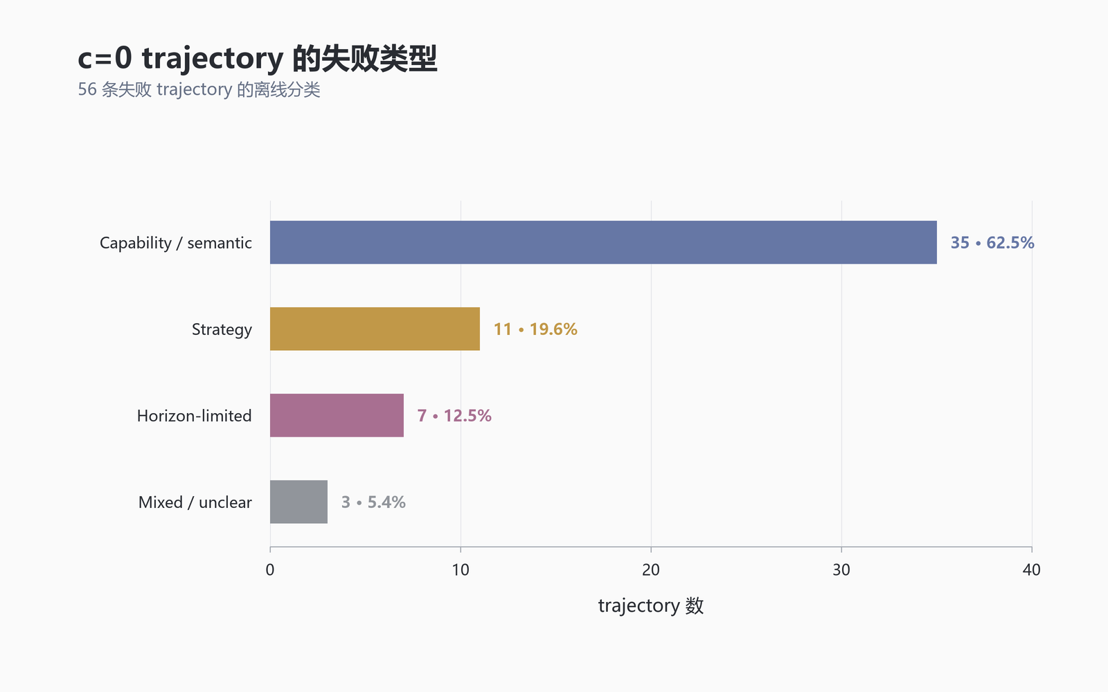
capability/semantic failures were the largest category among the 56 c=0 trajectories; 7 were classified as horizon-limited.
Chart guide: the horizontal axis counts trajectories. The four bars are capability/semantic, strategy, horizon-limited, and mixed/unclear failures; labels show counts and percentages from the offline classification.
Of the 56 trajectories, 22 hit the step limit, but only 7 were classified as horizon-limited. That classification additionally required edits near the end to remain localized, a nonempty Patch relevant to the issue, and tests that still produced new or improving feedback, without stagnation signals already dominating the run. Hitting the step limit alone does not establish that the failure was horizon-limited.
The capability/semantic category describes cases where the agent found relevant code and made relevant edits but did not satisfy the full software behavior constraints. It characterizes the current trajectory, not a ceiling on the model’s ability.
3.2 Three representative tasks
All seven tasks scored 0/8, but their failure processes differed. All 8 trajectories for astropy-7746 and flask-4992 were capability/semantic failures. xarray-3364 had 3 strategy failures, 3 horizon-limited failures, and 2 mixed cases. The remaining tasks had other combinations.
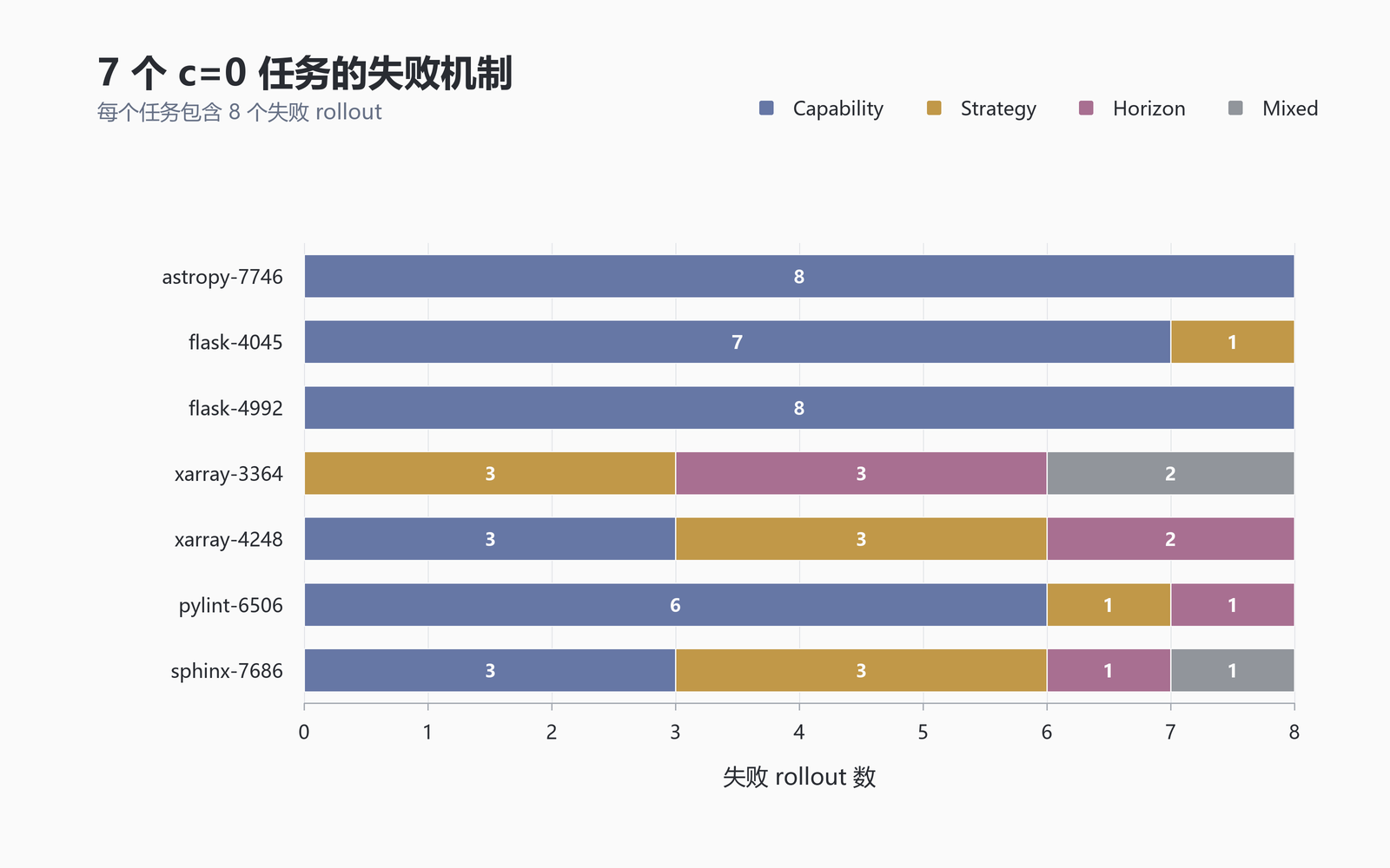
the 56 classification labels broken down by task, with 8 rollouts in each row.
Chart guide: the horizontal axis counts failed rollouts. Blue is capability/semantic, ochre is strategy, purple is horizon-limited, and gray is mixed/unclear.
The 8 flask-4992 rollouts quickly found Config.from_file, the relevant documentation, and tests. All called finish themselves, and none hit the 60-step limit. They tended to accept complete file-opening modes such as r and rb, while the actual call in the issue used mode='b'. The edit location was right, and some local tests passed. What they missed were the composition rules for file-opening modes and the public API semantics. The agents finished in 17 to 23 steps; raising the limit would not address this kind of omission.
All 8 xarray-3364 rollouts used the full 60 steps. Edits concentrated on concat.py, repeatedly dealing with variable discovery, the choice between merging and concatenation, dimensions, dtype promotion, and fill-value construction. Three were still making localized edits and receiving new or improving feedback at the end, so I classified them as horizon-limited. Another 3 were strategy failures and 2 were mixed. In the remaining processes, I saw repeated searching, rereading, and testing; some were still examining installed-package caches and external references late in the run. The final Patches remained incomplete or internally inconsistent. All 8/8 reaching the limit does not mean all 8/8 lacked enough execution steps.
All 8 astropy-7746 rollouts located the WCS array conversion and added an early return for empty input. Most trajectories received passing local-test feedback before calling finish themselves, and none hit the step limit. The final omissions involved constraints on output containers, shape semantics, axis counts, and ra_dec_order. They found the right code and passed local tests, but the full behavior still failed the verifier.
3.3 From adding steps to replanning
Before the failure analysis, I saw that failed trajectories ran longer on average and frequently hit the step limit, so I initially thought 60 steps wasn’t enough. When I examined the 7 c=0 tasks, though, 22 trajectories had hit the limit but only 7 looked more like horizon-limited cases. I began to realize that many failures were stuck on semantics, consistency across code paths, or search strategy—problems that simply running longer wouldn’t solve.
A longer execution budget might help a few trajectories. The 3 horizon-limited samples from xarray-3364 would be worth testing separately. But if every run were uniformly increased from 60 to 100 steps, trajectories already repeating searches, producing no new evidence, or drifting in scope would keep consuming budget too. Whether reward would improve remains unknown.
If I do another experiment, I’d try adaptive computation: selectively extend the budget when late edits remain focused and test feedback is still changing; trigger replanning or early stopping when searching and editing start repeating. Keeping the model, prompt, and tools unchanged and changing only the conditions for assigning extra steps would make the source of any change clearer.
3.4 Rejection Sampling
Among the 160 formal B trajectories, the verifier assigned reward=1 to 88 and reward=0 to 72. Rejection Sampling rejected the 72 failures, retained the 88 successes, and deduplicated Patches within each task to obtain 82 demonstration examples.
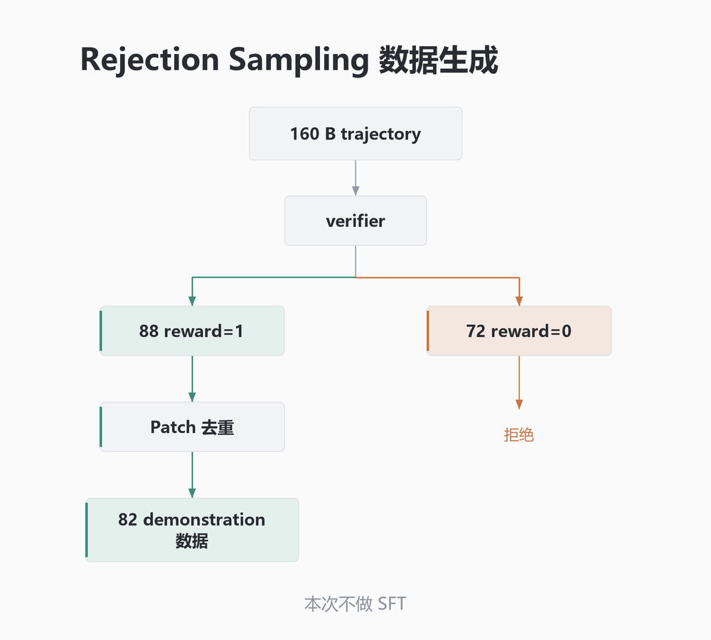
Generate → Verify → Filter; 160 trajectories became 88 successful records, then 82 demonstration examples after Patch deduplication.
Diagram guide: the verifier splits 160 B trajectories into 88 with reward=1 and 72 with reward=0. The latter are rejected; the former pass through Patch deduplication into 82 demonstration records. No SFT is performed in this Lab.
Filtering used only verifier results, with no manual selection. At this point, the Generate → Verify → Filter data-generation pipeline was working. I did not proceed to SFT: the harness, Agent Loop, Test-time Sampling, failure analysis, and Rejection Sampling this Lab set out to examine already had actual results. Adding a training stage would not answer the original three questions.
4. Looking back
The Pilot phase took a fair amount of time and tokens, but that expense was necessary. Pilot first eliminated harness problems involving output budgets, editing interfaces, and step limits, so Formal wouldn’t end up measuring faults in the experimental apparatus itself.
Formal’s most direct finding was that the Agent Loop substantially outperformed One-shot. With the same model, the same 20 SWE-bench Lite tasks, and a frozen experimental protocol, One-shot’s resolution rate was 20%, while Agent Loop Pass@1 was 55%. In other words, replacing static one-off inference with an Agent Loop that could actively retrieve code, use tools, run tests, and keep adjusting based on Observations improved single-run resolution by 35 percentage points. This was the clearest gain in the experiment.
The second finding was that Test-time Sampling helped, but its returns diminished quickly. The increase from 55% at Pass@1 to 65% at Pass@8 shows that running more independent rollouts did cover some single-run instability. But going from 4 rollouts to 8 added only 0.36 percentage points. Task-level results help explain this: 7 of the 20 tasks scored 8/8 and 7 scored 0/8, so most additional sampling gains came from the 6 in between. For the 0/8 tasks, I can only say that no success was observed in these 8 samples. I cannot conclude that further rollouts would necessarily be useless.
The third finding was that more computation did not automatically produce better results in this set of experiments. Failed trajectories ran longer on average and cost more. Of the 56 c=0 failures, 22 hit the step limit, but only 7 looked more like cases limited simply by execution length. Many trajectories had already found the relevant code and even passed some local tests, yet still missed API behavior, edge cases, output semantics, or consistency between code paths. At least on these results, uniformly raising max_steps above 60 does not look like the most promising first change.
So if I continue with another experiment, I’d optimize how computation is allocated: give more steps to trajectories still producing new feedback, trigger replanning when searches or edits start repeating, and stop early when needed. More than simply increasing rollouts or steps, what I now want to understand is: when is it worth continuing to compute, and when should I change direction?